PyPI:
Help!

General Instructions (for SOFCs)

Generic analysis

These instructions will walk through calculating the tortuosity for the two example files Electrolyte and Cathode. In general, the low-level methods _geo_dist(), _calc_interface(), _calc_tort(), and _calc_euc_x() do all the “heavy” lifting, while modules like tortuosity_from_labels_x() and run_full_analysis_lsm_ysz() wrap these methods into convenient higher-level interfaces.

1. Put the downloaded files into a directory accessible to Python, and fire up a Python session (Jupyter, notebook, etc.)

2. Import the module:

   >>> import fibtortuosity as ft
   

3. The following code will use the higher order function tortuosity_from_labels_x() to calculate the tortuosity in the x direction (perpendicular to the electrolyte boundary) The x direction function includes some additional code (compared to the y and z versions) that calculates the euclidean distance from the boundary of the bulk electrolyte, rather than simply from the edge of the volume.

   geo, euc, tort, and desc will contain the results of this calculation afterwards:

   >>> geo, euc, tort, desc = ft.tortuosity_from_labels_x('example_electrolyte.tif',
   ...                                                    'example_electrolyte_and_cathode.tif',
   ...                                                    'LSM',
   ...                                                     units='nm',
   ...                                                     print_output=True,
   ...                                                     save_output=False)
       Starting calculation on LSM in x direction.
       Loaded electrolyte data in 0:00:00.257833 seconds.
       Loaded cathode data in 0:00:00.252949 seconds.
       ImageDescription is: b'BoundingBox 3231.15 6462.29 0 4100.38 0 4000\n'
       Bounding box dimensions are: (3231.14, 4100.38, 4000.00) nm
       Voxel dimensions are: (16.16, 20.50, 20.00) nm
       Starting geodesic calculation at: 2016-04-05 15:52:57.412840
       Geodesic calculation took: 0:00:07.159744
       Calculating zero distance interface took: 0:00:00.207048
       Calculating euclidean distance took: 0:00:00.378937
       Calculating tortuosity took: 0:00:00.295921
       Total execution time was: 0:00:08.597359
   

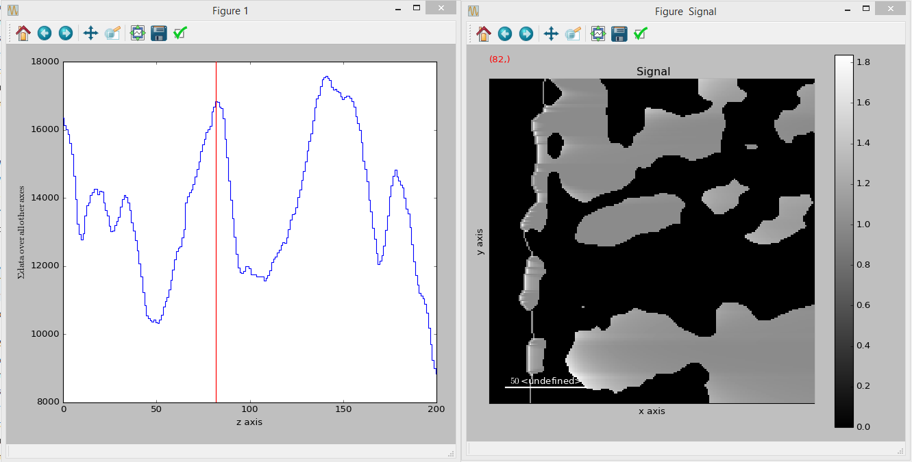
4. If HyperSpy is installed, it can be used to easily visualize the three-dimensional data that is produced as a result (example below is in Jupyter):

   >>> %matplotlib qt4
   >>> import hyperspy.api as hs
   >>> t_s = hs.signals.Image(tort)
   >>> for i, n in enumerate(['z', 'x', 'y']):
   ...     t_s.axes_manager[i].name = n
   >>> t_s.plot()
   

   

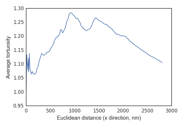
5. The tortuosity_profile() and plot_tort_prof() methods can be used to visualize the average tortuosity over a dimension:

   >>> t_avg, e_avg = ft.tortuosity_profile(tort, euc, axis='x')
   >>> ft.plot_tort_prof(t_avg, e_avg, 'x')
   

   

6. To save the results, a variety of export options are available. The average profiles can be easily saved using save_profile_to_csv(). The 3D tortuosity (or euclidean/geodesic distance) arrays can be saved as a 3D tiff using the save_as_tiff() method. Also, if HyperSpy is being used, it can save the data in the .hdf5 format (see its documentation for details). Furthermore, any of the Numpy methods for saving (such as save() or savez()) can be used directly on the resulting arrays.

   1. To save profile:

      >>> ft.save_profile_to_csv('profile.csv', e_avg, t_avg, 'x', 'LSM')
      

   2. To save tiff file:

      >>> # Using `desc` allows the file to be opened directly in Avizo
      >>> print(desc)
          b'BoundingBox 3231.15 6462.29 0 4100.38 0 4000\n'
      >>> ft.save_as_tiff('tortuosity.tif', tort, 'float32', desc)
          Writing TIFF records to tort_results.tif
          filling records:   100% done (12Mi+1003Ki+361 bytes/s)
          resized records: 31Mi+46Ki+716 bytes -> 8Mi+717Ki+565 bytes (compression: 3.59x)
      

      This gives you the following output: Tortuosity-profile and Tortuosity-data

Full Analysis

In my personal research, I more fully combined these methods into the highest-level function run_full_analysis_lsm_ysz(), so I could just run one function, walk away, and let it run. It has some additional useful features, like texting a number when it’s done or showing a browser notification. Also, it’s written with specific materials in mind, so it may take some tweaking to get it running for your specific needs, but I include it here as an idea of what can be done with the underlying code.

To do a full analysis of a sample (all phases and all directions), I would run something like the following, making sure that each of the files specified are in the current directory:

>>> import itertools
>>> import fibtortuosity as ft
>>> phases = ['LSM','YSZ','Pore']
>>> directions = ['x', 'y', 'z']
>>> for p, d in itertools.product(phases, directions):
...     ft.run_full_analysis_lsm_ysz(electrolyte_file="bulkYSZ.tif",
...                                  electrolyte_and_pore_file="bulkYSZandPRE.tif",
...                                  electrolyte_and_lsm_file="bulkYSZandLSM.tif",
...                                  electrolyte_and_ysz_file="bulkYSZandYSZ.tif",
...                                  date='2016-04-05',
...                                  phase=p,
...                                  direction=d,
...                                  npzfile=None,
...                                  units='nm',
...                                  delay=0,
...                                  calculate_all=True,
...                                  load_from_prev_run=False,
...                                  create_hspy_sigs=False,
...                                  save_avizo_tiff=True,
...                                  tort_profile=True,
...                                  save_tort_prof=True,
...                                  in_ipython=False)

After this has run, the directory will contain all the tortuosity data saved as .tif files, as well as all the average profiles for each phase and each direction, which can then be plotted/analyzed however is necessary.